Review Article
Institute of Micromechanics and Photonics, Warsaw University of Technology, św. A. Boboli 8, 02-525 Warsaw, Poland
Abstract. Shape measurement by optical methods is more and more often used in research both in human and veterinary medicine. As a result of the measurement, a set with marker positions in space or a cloud of points representing a scanned surface is obtained. The collected data contains useful information, but to extract it, it is necessary to process the data using appropriate algorithms. The aim of this study was to present the algorithms that the author used to process data for the purposes of analyzes which results and conclusions were included in four articles published earlier. The algorithms concern the determination and identification of markers on the body when measuring the posture of soccer players and the analysis of the cloud of points for determining the angles describing the base and surface of the hoof bones in the polar coordinate system. The measurement systems in which data were collected are also described. Sample results obtained with the presented analysis methods are shown. For the first case these are given directional views of the markers determined in 3D space, while for the other two the result containing information about the calculated angles in the form of a table and a graph are presented. The presented data processing methods and algorithms are not only applicable to the cases on which they were tested. Directly or after a small modification, they can be applied in another area.
Keywords: optical 3D measurements, cloud of points, markers,data analysis
Shape measurement in both human and veterinary medicine plays a role that cannot be overestimated in many cases. Knowing the correct size and shape of the organ that a specialist examines, he can diagnose the disease state and possible abnormalities in its structure for a specific case on the basis of the collected information. In the past, measurements were made only manually, often using specialized devices dedicated to a given measurement. Among others, the height, width, circumference of the organ as well as some characteristic angles described its shape were measured. Later, when x-rays were discovered, it became possible to measure also what is not directly visible to a person performing the test. With the development of radiological instruments, apart from typical x-ray, images from computed tomography, ultrasound and magnetic resonance imaging appeared. In the 70s of the last century, thanks to among others Takasaki's works optical methods of shape measurement joined this group [Takasaki 1970Takasaki, H. (1970). Moiré Topography. Appl. Optics, 9(6), 1467. https://doi.org/10.1364/AO.9.001467]. The aforementioned scientist, based on the Moiré effect, developed a system for registering the shape of the human body. Drerup [1981]Drerup, B. (1981). A procedure for the numerical analysis of moiré topograms. Photogrammetria, 36(2), 41–49. https://doi.org/10.1016/0031-8663(81)90016-8 also became interested in this technique, developing procedures related to the analysis of moiré fringes he simultaneously tried to apply them to that data which had Hierholzer and Frobin [1980]Hierholzer, E., Frobin, W. (1980). Methods of Evaluation and Analysis of Rasterstereographic Surface Measurements. Int. Arch. Photogram. 23(5), 329–337. Google Scholar obtained in parallel in rasterography. With the development of digital cameras and projection systems, the Moiré-based methods have lost their relevance, but the experience and knowledge of analyzing human body topography have proved useful also in raster stereography. Drerup and Hierholzer [1987]Drerup, B., Hierholzer, E. (1987). Automatic localization of anatomical landmarks on the back surface and construction of a body-fixed coordinate system. J. Biomech., 20(10), 961–970. https://doi.org/10.1016/0021-9290(87)90325-3 joining their forces developed, among others, a method for automatic localization of some characteristic points on the human back surface.
Techniques based on fringe analysis have undergone significant development since Takasaki's time [Bartol et al. 2021Bartol, K., Bojanic, D., Petkovic, T., Pribanic, T. (2021). A Review of Body Measurement Using 3D Scanning. IEEE Access, 9, 67281–67301. https://doi.org/10.1109/ACCESS.2021.3076595]. Progress has been made in various fields. The measurement frequency was increased and now reaches many thousands of Hz, for example Hyun et al achieved a recording frequency of 10,000 Hz [Zhang 2018Zhang, S. (2018). High-speed 3D shape measurement with structured light methods: A review. Optics Lasers Engin., 106, 119–131. https://doi.org/10.1016/j.optlaseng.2018.02.017]. A number of modifications were proposed regarding a set of projected fringes, these solutions differ in the designed pattern and the number of projected images [Geng 2011Geng, J. (2011). Structured-light 3D surface imaging: a tutorial. Advances in Optics and Photonics, 3(2), 128. https://doi.org/10.1364/AOP.3.000128, Huang et al. 2021Huang, X., Cao, Y., Yang, C., Zhang, Y., Gao, J. (2021). A Single-Shot 3D Measuring Method Based on Quadrature Phase-Shifting Color Composite Grating Projection. Appl. Sci., 11(6), 2522. https://doi.org/10.3390/app11062522, Ye and Zhou 2021Ye, J., Zhou, C. (2021). Time‐resolved coded structured light for 3D measurement. Microw. Optical Techn. Let., 63(1), 5–12. https://doi.org/10.1002/mop.32548].
3D scanners used in medical science work in various configurations. Both handheld and stationary scanners are used. The possibility of using selected scanners to record the shape of the upper limb, in a form of review article, was presented by Paoli et al. [2020]Paoli, A., Neri, P., Razionale, A.V., Tamburrino, F., Barone, S. (2020). Sensor Architectures and Technologies for Upper Limb 3D Surface Reconstruction: A Review. Sensors, 20(22), 6584. https://doi.org/10.3390/s20226584.
Optical 3D scanners are used not only to register stationary objects, but also objects in motion. The sequence of a person's movement, without the use of markers, can be recorded for example with a multidirectional system built by the Sitnik's group [Sitnik et al. 2019Sitnik, R., Nowak, M., Liberadzki, P., Michoński, J. (2019). 4D scanning system for measurement of human body in motion. Electron. Imag., 2019(16), 2–1-2–7. https://doi.org/10.2352/ISSN.2470-1173.2019.16.3DMP-002].
About the undoubted advantages, as well as the limitations and possibilities of using 3D scanners in medical practice one can learn from publication of Haleem and Javaid [2019]Haleem, A., Javaid, M. (2019). 3D scanning applications in medical field: A literature-based review. Clin. Epidem. Global Health, 7(2), 199–210. https://doi.org/10.1016/j.cegh.2018.05.006.
A technique much older than stripe techniques is photogrammetry. Some references to it can be found already in the notes of Leonardo da Vinci from 1480 [Doyle 1964Doyle, F. (1964). The Historical Development of Analytical Photogrammetry. Photogram. Engin., 30(2), 259–265. Google Scholar], but not he is called the father of photogrammetry, but Aimé Laussedat, who was the first to use photographs of an area to create its topography [Birdseye 1940Birdseye, C.H. (1940). Stereoscopic Phototopographic Mapping. Ann. Assoc. Am. Geogr., 30(1), 1–24. https://doi.org/10.1080/00045604009357193]. Visual analysis based on comparison of characteristic points visible on two images is very laborious, therefore this technique, like other optical techniques, experienced a real renaissance with the development of digital methods of image recording and analysis. In the context of medical research, Mannsbach was the first person to apply stereo photogrammetry in this area in 1922 [Burke and Beard 1967Burke, P.H., Beard, L.F.H. (1967). Stereophotogrammetry of the face. Am. J. Orthodont., 53(10), 769–782. https://doi.org/10.1016/0002-9416(67)90121-2].
The undoubted advantage of this type of solution, from the point of view of today's applications, is its simplicity and relatively low cost of a device its usage. A simple photogrammetric system can be set up, for example, from two cameras. In the case of the aforementioned stereopair and time-varying objects, it is necessary to ensure synchronization between the two recording devices, so that the pictures from both cameras represent the state of the object from the same moment. An extension of this idea is, for example, the quite widely used Vicon system, which the authors intended was created as a system for measuring human gait [Sutherland 2002Sutherland, D. (2002). The evolution of clinical gait analysis. Gait \& Posture, 16(2), 159–179. https://doi.org/10.1016/S0966-6362(02)00004-8]. Not only large movements can be monitored in this way, but also small ones, e.g. at analyzing of postural stability [Ould-Slimane et al. 2017Ould-Slimane, M., Latrobe, C., Michelin, P., Chastan, N., Dujardin, F., Roussignol, X., Gauthé, R. (2017). Noninvasive Optoelectronic Assessment of Induced Sagittal Imbalance Using the Vicon System. World Neurosurgery, 102, 425–433. https://doi.org/10.1016/j.wneu.2017.03.099].
Photogrammetric techniques also include a method called Structure from Motion (SfM) [Granshaw 2018Granshaw, S.I. (2018). Structure from motion: origins and originality. The Photogrammetric Record, 33(161), 6–10. https://doi.org/10.1111/phor.12237]. Images used by this method can be recorded with one or more unsynchronized cameras. The method is suitable for registering the shape of static objects. In medicine, for example, the skull is such an object. Measurements of infants' heads and analysis of the obtained results allowed Barbero-García et al. [2019]Barbero-García, I., Lerma, J.L., Miranda, P., Marqués-Mateu, Á. (2019). Smartphone-based photogrammetric 3D modelling assessment by comparison with radiological medical imaging for cranial deformation analysis. Measurement, 131, 372–379. https://doi.org/10.1016/j.measurement.2018.08.059 to conclude that it is possible to assess the infants' skull on the basis of photogrammetric data calculated from images recorded with a cheap smartphone, and the obtained results do not differ from those provided by radiological methods. Using this technique one can also reconstructs microscopic objects. Due to the fact that the depth of field for a single microscopic image is small, collecting a series of images for each direction of registration and use a technique that basing on the series allows to increase the depth, e.g. Focus Stacking, is a solution that gives the entire registered object is well visible on the resulting image, and such image can be loaded to the SfM [Paśko et al. 2020Paśko, S., Sutkowski, M., Bakanas, R. (2020). Use of focus stacking and SfM techniques in the process of registration of a small object hologram. Chin. Optics Let., 18(6), 060901. https://doi.org/10.3788/COL202018.060901].
In parallel, both algorithms and software for data processing are developed either for data in a form of clouds of points or sets of independent points. For example, in the area of the torso, the work focuses mainly on determining the profile of the spine [Poredoš et al. 2015Poredoš, P., Čelan, D., Možina, J., Jezeršek, M. (2015). Determination of the human spine curve based on laser triangulation. BMC Med. Imag., 15(1), 2. https://doi.org/10.1186/s12880-015-0044-5, Little et al. 2019Little, J.P., Rayward, L., Pearcy, M.J., Izatt, M.T., Green, D., Labrom, R.D., Askin, G.N. (2019). Predicting spinal profile using 3D non-contact surface scanning: Changes in surface topography as a predictor of internal spinal alignment. PLOS ONE, 14(9), e0222453. https://doi.org/10.1371/journal.pone.0222453, Roy et al. 2019Roy, S., Grünwald, A.T.D., Alves-Pinto, A., Maier, R., Cremers, D., Pfeiffer, D., Lampe, R. (2019). A Noninvasive 3D Body Scanner and Software Tool towards Analysis of Scoliosis. BioMed Res. Int., 2019, 1–15. https://doi.org/10.1155/2019/4715720],and characteristic points for this surface [Michoński et al. 2012Michoński, J., Glinkowski, W., Witkowski, M., Sitnik, R. (2012). Automatic recognition of surface landmarks of anatomical structures of back and posture. J. Biomed, Optics, 17(5), 056015. https://doi.org/10.1117/1.JBO.17.5.056015]. For the determination of the spine line, in the severe scoliosis cases, when it is impossible to do only on the basis of the cloud of points, a method that uses both a cloud of point and a frontal x-ray image is used [Paśko and Glinkowski 2020Paśko, S., Glinkowski, W. (2020). Combining 3D Structured Light Imaging and Spine X-ray Data Improves Visualization of the Spinous Lines in the Scoliotic Spine. Appl. Sci., 11(1), 301. https://doi.org/10.3390/app11010301]. When the works concern the limbs, their movement is usually analyzed [Rocha et al. 2018Rocha, A.P., Choupina, H.M.P., Vilas-Boas, M. do C., Fernandes, J.M., Cunha, J.P.S. (2018). System for automatic gait analysis based on a single RGB-D camera. PLOS ONE, 13(8), e0201728. https://doi.org/10.1371/journal.pone.0201728, Zhang et al. 2018Zhang, M., Artan, N., Gu, H., Dong, Z., Burina Ganatra, L., Shermon, S., Rabin, E. (2018). Gait Study of Parkinson’s Disease Subjects Using Haptic Cues with A Motorized Walker. Sensors, 18(10), 3549. https://doi.org/10.3390/s18103549, Zago et al. 2020Zago, M., Luzzago, M., Marangoni, T., De Cecco, M., Tarabini, M., Galli, M. (2020). 3D Tracking of Human Motion Using Visual Skeletonization and Stereoscopic Vision. Front. Bioengin. Biotech., 8. https://doi.org/10.3389/fbioe.2020.00181].
Unfortunately, not every article formula allows for an in-depth presentation of an underlying algorithm used to process collected data. Due to the profile of readers of a given journal, content that would be boring or incomprehensible to them is often avoided. For this reason this publication describes the algorithms that have been used to process data in already published articles, which concerned the study of the body posture in soccer players [Sutkowski et al. 2017Sutkowski, M., Paśko, S., Żuk, B. (2017). A study of interdependence of geometry of the nuchal neck triangle and cervical spine line in the habitual and straightened postures. J. Anatom. Soc. India, 66(1), 31–36. https://doi.org/10.1016/j.jasi.2017.05.006, Żuk et al. 2019Żuk, B., Sutkowski, M., Paśko, S., Grudniewski, T. (2019). Posture correctness of young female soccer players. Sci. Rep., 9(1), 11179. https://doi.org/10.1038/s41598-019-47619-1] and angles describing the base and surface of hoof bones [Paśko et al. 2017Paśko, S., Dzierzęcka, M., Purzyc, H., Charuta, A., Barszcz, K., Bartyzel, B.J., Komosa, M. (2017). The Osteometry of Equine Third Phalanx by the Use of Three-Dimensional Scanning: New Measurement Possibilities. Scanning, 2017, 1–6. https://doi.org/10.1155/2017/1378947, Dzierzęcka et al. 2020Dzierzęcka, M., Paśko, S., Komosa, M., Barszcz, K., Bartyzel, B.J., Czerniawska-Piątkowska, E. (2020). Impact of Horse Age and Body Weight on the Angle Between the Parietal Surface of the Coffin Bone and the Ground. Pak. J. Zool., 53(3), 895–901. https://doi.org/10.17582/journal.pjz/20190429200419]. In the following text, the individual processing steps are described in a practical way, when start from the raw data and end with the calculated values.
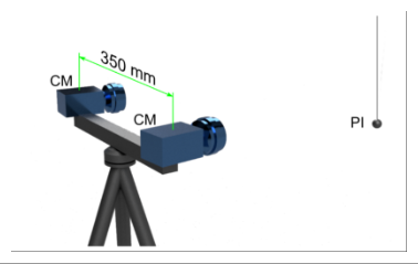
The measurement system and data analysis procedures were created to measure the distribution of markers on the body of the examined person in 3D space. The measuring stand was built on the basis of two cameras with an image sensor in the APS-C format and the number of pixels approximately equal to 16 million. The lenses used had a focal length of 30mm. The base distance for the stereo pair was 350 mm. The cameras were mounted on a rigid beam, which in turn was mounted on a photographic tripod. The devices were mutually synchronized. The measurement system is schematically shown in Fig. 1.
The measuring area began about 1500 mm from the measurement system. Its dimensions were approximately 600×500×1200 mm. The area was calibrated using a calibration board consisting of alternating black and white squares, 8 horizontally and 12 vertically, sized 50×50 mm. The applied calibration procedure was modeled on the code from the book by Bradski and Kaehler [2008]Bradski, G., Kaehler, A. (2008). Learning OpenCV: Computer Vision with the OpenCV Library (1st ed.). O’Reilly Media. Google Scholar, changing used functions options and values of their parameters. The OpenCV (version 3.0.0) function findChessboardCorners was used to find the inside corners in the board by selecting the option that forces the gamma normalization of the image before the next operation, which in this case was an adaptive, based on the mean value in the vicinity of the analyzed pixel threshold. After determining the positions of the corners of the chessboard elements, another function of the package was launched, cornerSubPix, which using those information iteratively calculated exact positions of the corners.
|
Fig. 1. The measuring stand used in the static body posture examination, CM – camera, PI – plumb indicator |
The principle of this function is described in the article by Förstner and Gülch [1987]Förstner, W., Gülch, E. (1987). A fast operator for detection and precise location of distinct points, corners and center of circular features. Proc. of ISPRS Inter-Commission Conference on Fast Processing of Photogrammetric Data, 281–305. Google Scholar. Half the search window size assumed for this algorithm is 21×21. The size of the dead region was not declared, so pixel values from the center of the search window were also used in the calculations. A maximum of 100 iterations and a minimum change between iterations (epsilon) at the level of 10–4 were assumed. Knowing the positions of corresponding points of the pattern visible in the images taken by the both cameras, the stereoCalibrate function was used to calculate the internal parameters of each camera of the stereopair and the external parameters determining their relative position and orientation. The tangential distortion factor for both cameras was fixed at zero, as it was done with the factors K4, K5 and K6. The maximum number of iterations for this algorithm was set to 400 and the epsilon parameter to 10–5.
Printed black and white markers were used in the study. They were 10mm in diameter. The outer part of the marker surface was black, in the central part there was a white circle with a diameter of 3 mm. Before the study, the markers were stuck to the body of volunteers, which after that were asked to take a place within the measurement space. Then, the sequences of photos were taken with cameras constituting a stereopair. Each pair of photos contained a different posture. Initially, attempts were made to find the markers automatically, but due to the underwear, skin discoloration and shadows, the developed procedures returned additional, incorrect points. The identification and removal of them was time-consuming. Therefore, it was decided to use a different method, partly manual, which would ultimately speed up the processing of a large set of photos. For this purpose, color photos were converted to black and white and the internal areas of markers were manually marked with a graphics program, filling them with red. The images were rectified using OpenCV stereoRectify, initUndistortRectifyMap and remap functions. The first two functions use data calculated during the calibration. The saved resulting images, it was decided, to further process in the Matlab environment due to the higher speed of creating of prototype procedures resulting from, inter alia, lack of requirement of compilation of all the code after changing it.
RGB images in which each color channel was encoded on 8 bits were binarized. Assuming that the pixel color at a point i is described by the RiGiBi triad, the idea of the binarization used can be described as:
$$W_i=\left\{\begin{matrix} 1 :(R_i-G_i)>T \\ 0 : others \end{matrix}\right.$$
where:
\( W_i \) - a binary distribution, with 1 (true), specifying the pixels within the marker, and 0 (false), the rest,
\( T \) - the cutoff level experimentally set to 40.
To remove small artifacts, the bwareaopen function was used, which removes all pixel groups where their number is smaller than the assumed one. It was assumed that the limit value will be 5. In the next step, the bwconncomp function was used, which returned the elements composed of connected pixels as a result. For each element the regionprops function was used to determine its basic parameters. Since the markers were circular in shape, the coordinates of the centroid describing each element were taken for further analysis.
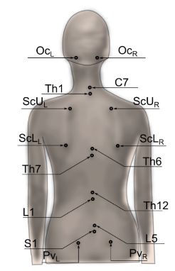
The distribution of markers located at characteristic points on the back of an exemplary examined person is presented in Fig. 2. OcL and OcR are the mastoid processes, C7, Th1, Th6, Th7, Th12, L1, L5, and S1 are the marked selected spinous processes of the spine. ScUL, ScUR, ScLL, ScLR are the right and left upper and lower scapular angles, respectively. PvL, PvR are the right and left iliac crest. The position of these points changes slightly depending on the position the person takes.
|
Fig. 2. Schematic distribution of markers at characteristic, marked points, on the body of a volunteer (Figure based on research by Paśko et al., years 2017–2019) |
Since both the algorithm for calculating the position of a point in space needs paired points from both cameras, as well as further analyzes require linking the point position with an identifier that gives it meaning in the context of the determined medical parameters, an algorithm for their identification has been developed. Assuming that the x-axis of the coordinate system reflects the position of a point horizontally and the z-axis vertically, the first operation that is performed on the set of points representing the centers of markers is their sorting under the z-axis. Image analysis indicates that the z-axis coordinates of the pelvic crest points will be smaller than the others. To separate PvL points from PvR, their x-axis coordinates should be compared. The coordinate of the PvL(x) point is smaller than PvR(x). After removing them from the analyzed set, points from Th12, L1, L5 to S1 are identified based on the z-axis coordinate. Subsequent points above Th12 cannot be identified in this way because the position of the points ScLL, ScLR in the z-axis is very close to the points Th6 and Th7. Therefore, the two points with the highest coordinate are selected from the remaining points in the set. They are OcL and OcR. Their right and left distinction is based on the same comparison used for PvL and PvR. After removing these points from the analyzed set, two more points, C7 and Th1, are identified by their position in the z-axis. These points are also removed and then in the set the largest values of coordinates in the z-axis will have the points ScUL, ScUR, z which were separated by the same principle as the already mentioned PvL i PvR. After this operation, only four points ScLL, ScLR, Th6 and Th7 remain in the analyzed set. The point ScLL is identified as the one with the smallest coordinate value in the x-axis, and the point ScLR with the largest. After removing them, Th6 and Th7 are identified by their z-axis coordinate.
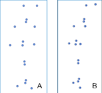
Once the markers for the left and right stereo pair cameras are marked, they are entered as pairs of coordinates into the perspectiveTransform procedure that is part of OpenCV, which calculates the coordinates of a point in space based on its position and the separation of its representation in the images from both cameras. The result of this operation can be seen in Fig. 3, where the points are presented as they look in the view directly taken the reconstruction and when they are rotated by an angle of 45° with respect to the z-axis.
|
Fig. 3. Reconstruction of the characteristic points on the body of a volunteer: (A) direct view, (B) view rotated 45° about the z-axis (Figure based on research by Paśko et al., years 2017–2019) |
Since the angles of straight lines passing through selected points in relation to the vertical and horizontal are important information, an additional calibration element was the leveling of the system on the basis of additional images acquired from the cameras, which showed a rope on the end of which a weight was hung. Two markers were placed on the rope so that the parameters of the straight line passing through them could be determined. This in turn allowed to determine the transformation that allowed to rotate the reconstructed data so that it corresponded to the actual position of the subjects' bodies in relation to the vertical. This action eliminates the need to ensure that the cameras are mounted precisely in relation to the supporting element and that the system is accurately leveled afterwards prior to the measurement.
The developed algorithm, in the presented version, was used to carry out the assessment of body posture of footballers in the frontal view from the back side and to compare the determined parameters with the control group [Żuk et al. 2019Żuk, B., Sutkowski, M., Paśko, S., Grudniewski, T. (2019). Posture correctness of young female soccer players. Sci. Rep., 9(1), 11179. https://doi.org/10.1038/s41598-019-47619-1]. Prior to the aforementioned study, the algorithm, in a simplified form, that did not take into account the lower scapular angles, was used to evaluate the posture of a group of the volunteers [Sutkowski et al. 2017Sutkowski, M., Paśko, S., Żuk, B. (2017). A study of interdependence of geometry of the nuchal neck triangle and cervical spine line in the habitual and straightened postures. J. Anatom. Soc. India, 66(1), 31–36. https://doi.org/10.1016/j.jasi.2017.05.006].
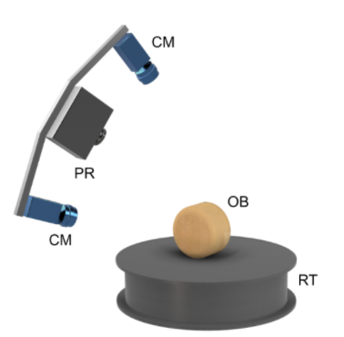
The measurement system consisted of a rotary table mounted on a common base and a robotic arm on which the 3D scanner head was mounted. The use of a robot in the scanning system simplifies the procedure of positioning the scanner in relation to the measured object, but in the scanning process itself it plays no other role. Therefore, the measurement system can be simplified and presented as shown in Fig. 4. The working principle of the scanner does not differ from other devices of this type and come down to the fact that the measured object OB is illuminated by the projector PR with a sequence of appropriately prepared patterns. The projected patterns are observed from another place, in this case located above and below the projector by two cameras. The method used was based on the solution proposed in the paper by [Sitnik et al. 2002Sitnik, R., Kujawińska, M., Woźnicki, J. M. (2002). Digital fringe projection system for large-volume 360-deg shape measurement. Optical Engin., 41(2), 443. https://doi.org/10.1117/1.1430422].
The base between the cameras was 500 mm, between them, in the center, the projector was placed. The angle between the optical axis of the projector and the optical axis of each camera was approximately 60°. The system used 2 Mpix color cameras and an HD Ready projector. The calibrated measurement volume measured 180×180×100 mm. The system was calibrated so that one of the coordinate axes in the resulting cloud passed through the rotation axis of the stage, which platform had been previously leveled. Since each camera was a separate scanning system with a common projector, two independent point clouds were collected from one direction, which were later combined based on the information from the spatial calibration. The axial accuracy for the scanners as well as their lateral resolution was 0.1 mm.
It was determined that the object would be measured every 15°, which gave 24 measurements for a full rotation of the table. Positioning of the rotary stage was done to an accuracy of 0.025°. The leveling of the stage and the calibration that forced the vertical axis of the coordinate system to overlap meant that the resulting clouds of points were already initially composed. Small errors in transformations between clouds were determined using the RANSAC algorithm and corrected.
|
Fig. 4. Diagram of a two-camera 3D scanning system: CM – camera, PR – projector, RT – rotary table, OB – measured object |
|
Fig. 5. Sample measurement result for the coffin bone after initial cloud preprocessing (Figure based on research by Paśko et al., years 2016–2020) |
|
Fig. 6. Projection of a sample cloud of the coffin bone onto the xy plane (Figure based on research by Paśko et al., years 2016–2020) |
|
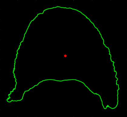
Fig. 7. Contour of a cloud of points of the coffin bone projected onto the xy plane, with the center of gravity, calculated for the cloud, highlighted in red (Figure based on research by Paśko et al., years 2016–2020) |
|
Fig.
8. The
method of determining value of angles for the edge line for a
coffin bone, α – calculated angle (Figure based on
research by Paśko et al., years |
As the color of the scanned bones was not identical, therefore, during each measurement, experimental selection was made of the appropriate gain and shutter speed values so that the collected fringe image had the highest possible contrast and was not overexposed or underexposed anywhere.
The output point cloud, besides being noisy, also contained additional elements that were present in the measurement volume during scanning or were the result of cloud distortions near areas where one of the images collected by a given camera was overexposed. These erroneous or unnecessary data had to be manually removed before further analysis could be performed. This was done in FRAMES software developed at the Department of Virtual Reality Technology of the Warsaw University of Technology.
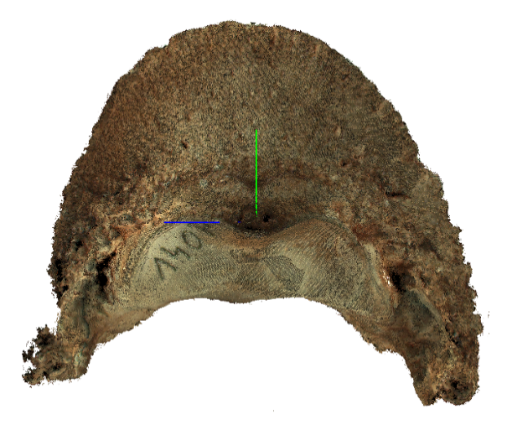
It should be mentioned that the bones were positioned during scanning so that their orientation in the xy plane was approximately the same. The y-axis of the coordinate system was oriented in the anterior-posterior direction of the bones, while the x-axis passed through the lateral planes of the bones and was approximately parallel to the plane located between the place where the coffin bone joins the short pastern bone and the place where it joins the navicular bone. The orientation of the bones supported by their natural elements, with respect to the z-axis, was assured by the leveling of the stage and appropriate positioning ensured that this axis passed approximately through the extremity of the extensor process.Any orientation errors visible in the xy plane during processing were initially corrected in FRAMES. Data obtained after this stage were saved in ply format, which is a format accepted both by FRAMES and Matlab, in which a large part of analyses were performed.
The result of an example measurement after preprocessing and noise filtering can be seen in Fig. 5. Based on the obtained data, analyses of the angular distribution of change of the shape of the edge of the base of the coffin bones [Paśko et al. 2017Paśko, S., Dzierzęcka, M., Purzyc, H., Charuta, A., Barszcz, K., Bartyzel, B.J., Komosa, M. (2017). The Osteometry of Equine Third Phalanx by the Use of Three-Dimensional Scanning: New Measurement Possibilities. Scanning, 2017, 1–6. https://doi.org/10.1155/2017/1378947] and the mutual angular position of a lateral planes of the mentioned bones [Dzierzęcka et al. 2020Dzierzęcka, M., Paśko, S., Komosa, M., Barszcz, K., Bartyzel, B.J., Czerniawska-Piątkowska, E. (2020). Impact of Horse Age and Body Weight on the Angle Between the Parietal Surface of the Coffin Bone and the Ground. Pak. J. Zool., 53(3), 895–901. https://doi.org/10.17582/journal.pjz/20190429200419] were performed. The algorithms that were used for this purpose are described in turn below.
As the platform on which the bone was scanned was leveled, the operation of projecting onto the xy plane was reduced to reducing the data dimension from 3D to 2D by setting to zero the z coordinate of all points. The resulting distribution was sampled by a raster. The raster size was assumed to be 0.1 mm, which was the same as the lateral resolution of the scanner. Since the sizes of all bones were known it was possible to establish a common size for all of them. The assumed size for the raster data was 1400×1200 pixels . It was slightly larger than it would result from calculations based on the maximum size of the largest object in the xy plane. The established reserve guaranteed that if there was a need to analyze a new, larger bone, its image would also have a chance to be calculated by this algorithm without making any changes.
In order to discretize the resulting two-dimensional distribution, the maximum and minimum values in each of the two dimensions were determined, and then a grid of points equidistant from each other by 0.1 mm was created on this basis. The grid constituted one parameter of Matlab's knnsearch function, another was the point cloud. After processing and manual removal of any remaining noise and artifacts after the previous manual editing, a two-dimensional image representing the projection of the point cloud onto the xy plane was obtained (Fig. 6).
In the next step, a closure operation was performed on the binary image to modify the value in pixels came from the projection of the cloud on the xy plane, so that it represented a reasonably continuous space in terms of value.
In order to ensure the best possible alignment between the right and left bones, a copy of the image of the right bone was made, rotated horizontally, and then the image of the left bone was superimposed on this resulting image. If it was noticed that there was a difference in orientation between the images, the image of the right bone was manually rotated and shifted to compensate for this difference.
After this operation, the center of gravity of the image of each bone was calculated. This point became the center of the polar coordinate system, and this information was used in a later step. Then the Matlab function bwmorph with parameter “remove” was performed to remove all internal pixels in the image. Only the contour remained. Any internal contours resulting from unscanned areas were removed manually. The final result is shown in Fig. 7. The not scanned small areas appeared where there were holes in the bone. These holes are largely remnants of blood vessels that ran there in the past. The resulting contour was transformed into the aforementioned polar system, in which 9 measuring points were determined within an angle of ±90°, spaced 22.5° apart. Each measurement point was assigned a section of the contour which extended in its vicinity within ±22.5° . The number of points and the angular range were chosen experimentally in order to minimize the influence of contour distortions resulting from soft tissue removal. After the calculated contour sections were transformed to Cartesian coordinates, Matlab's polyfit function was used to fit the straight line to a given contour section, and then the angle between this line and the line passing through the center of gravity and the current measurement point was calculated. The above idea is schematically shown in Fig. 8. The calculated distribution of angles for successive measurement points counted from the left, according to the clockwise direction is shown in Table 1.
Table 1. Calculated value of a coffin bone base angle at selected measurement points for an exemplary bone (Table based on research by Paśko et al., years 2016–2020) |
|||||||||
Measurement point |
1 |
2 |
3 |
4 |
5 |
6 |
7 |
8 |
9 |
Angle [°] |
16.7 |
3.8 |
–0.9 |
3.0 |
5.7 |
6.9 |
2.8 |
–8.0 |
–22.6 |
In order to see the distribution of angles formed by the surface of the coffin bone with the xy plane for one case, it was decided to create a triangle mesh from the cloud of points. Conversion was performed in CloudCompare software using algorithm based on solving Poisson's equations with Naumann's boundary condition. The obtained mesh was loaded into Blender software, where the fragment shader script was used to modify the texture color of each triangle composing the object, and binding the color directly to the angle that the normal of the analyzed triangle forms with z axis. The result is shown in Fig. 9.
|
Fig. 9. Visualization of the distribution of angles on the coffin bone surface in (A) top view, (B) front view, and (C) side view (Figure based on research by Paśko et al., years 2016–2020) |
|
Fig. 10. Visualization of the coffin bone surface section taken for counting lateral surface angles in (A) top view, (B) front view, and (C) side view (Figure based on research by Paśko et al., years 2016–2020) |
|
Fig. 11. Distribution of the inclination angle of the lateral surface of the coffin bone as a function of the azimuthal length (Figure based on research by Paśko et al., years 2016–2020) |
The performed try showed that the distribution of angles for most of the surfaces is in the range of about 30° (50–80°). On the other hand, there are no noticeable locations that are clearly different from the others and represent an interesting detail worth analyzing.
It was noticed, however, that if for a given bone the areas belonging to and adjacent to the palmar process and the extensor process were neglected, the change in the angle of inclination of the bone surface was a slowly varying function. Since the angle of this area for successive objects varied, it was decided to see if it correlates with the parameters describing the case. The angle measured for these surfaces in relation to the vertical depends on the natural support points of the bones they contact the stage surface, so in order to minimize the risk of obtaining erroneous results, it was decided to calculate the angle between the two lateral bone surfaces and use this parameter in subsequent statistics.
Two consecutive conversions were performed using CloudCompare. The first converted all clouds of points to triangle grids, and then what was obtained was converted back to clouds of points. This action was dictated by the fact that converting the cloud to a mesh eliminated any loss in the cloud and reduced noise, while returning to point cloud form allowed us to use elements of the computational script created for the analysis presented in the previous section. However, before this procedure was run on the data, areas belonging to, and close to, the palmar process and the extensor process were removed from the clouds (Fig. 10). The origin of the coordinate system, as mentioned earlier was located at the highest point of the extensor process. In the first step, after loading the cloud, the coordinates of the points were transferred to the spherical coordinate system, with the center at the above-mentioned point. An angular area equal azimuthally to 7/12 π radians was considered in the calculations, which in terms of degrees, in the Cartesian system, in the xy plane gave an area of ±105° with respect to the y axis. This area was divided into 100 parts. For each part of the cloud, after converting it into Cartesian coordinates, the center of gravity was determined, which coordinates were subtracted from the coordinates of each point. The Matlab function svd was then used to perform a decomposition of the matrix into singular values to calculate a straight line that the best fits the data. The last operation was to calculate the angle between this line and the axis of the spherical coordinate system. In this way, the distribution of the angles of the lateral coffin bone was obtained. An example is shown in Fig. 11. In the case of the above distribution, due to the aforementioned limitations resulting from bone positioning, in the article in which they were compared and correlated with the age and weight of the horse [Dzierzęcka et al. 2020Dzierzęcka, M., Paśko, S., Komosa, M., Barszcz, K., Bartyzel, B.J., Czerniawska-Piątkowska, E. (2020). Impact of Horse Age and Body Weight on the Angle Between the Parietal Surface of the Coffin Bone and the Ground. Pak. J. Zool., 53(3), 895–901. https://doi.org/10.17582/journal.pjz/20190429200419], only two areas within the azimuthal length <–105, –85> and <105, 85> were taken into account.
Optical scanning systems are non-invasive, non-contact and fast. For this reason, more and more centers are choosing to use them. Depending on the system with which the data has been collected, its output may be in a form of two-dimensional images, sets of points representing detected markers, point clouds or polygonal grids (usually triangular grids).
This paper presents three cases of spatial data analysis made for medical and veterinary analysis. It is shown how to analyze data from stereometric systems that use markers, as well as an approach suitable for data recorded with systems based on raster projection, or other technique that returns a cloud of points as a result of its work.
In the first case, the processing began with the analysis of images recorded by cameras. It was followed by the identification of pairs of markers, and determination of their position in 3D space. During the analysis of 2D images, which aimed to determine the position of black and white markers, the most work was done manually. In future studies, we will certainly use markers with color significantly different from the color of the human skin. In this case, the entire processing can be completely automated.
For point cloud analysis, the steps from its registration to the determination of the desired value were described in detail. The transition with data to the spherical space made it possible to easily separate fragments of the cloud, which could later be analyzed independently.
The presented algorithms, as well as their fragments, can be treated as a useful hint in the analysis of similar objects.
I would like to express my sincere thanks to Beata Żuk, Ph.D., Małgorzata Dzierzęcka-Gappa, Ph.D., Bartłomiej Jan Bartyzel, Ph.D., Marek Sutkowski, Ph.D., and all the others who took part in the research, the result of which is the publication of the global effects of these works.
Received: 13 Feb 2021
Accepted: 15 May 2021
Published online: 22 Jul 2021
Accesses: 994
Paśko, S., (2021). Optical 3D scanning methods in biological research - selected cases. Acta Sci. Pol. Zootechnica, 20(1), 3–14. DOI: 10.21005/asp.2021.20.1.01.